DSP Using MATLAB

1. DFT of given sequence using MATLAB

Fourier analysis is a family of mathematical techniques, all based on decomposing signals into sinusoids. The discrete Fourier transform (DFT) is the family member used with digitized signals. A signal can be either continuous or discrete, and it can be either periodic or Aperiodic. The combination of these two features generates the four categories, described below

·         Aperiodic-Continuous

This includes, decaying exponentials and the Gaussian curve. These signals extend to both positive and negative infinity without repeating in a periodic pattern. The Fourier Transform for this type of signal is simply called the Fourier Transform.

·         Periodic-Continuous

This includes: sine waves, square waves, and any waveform that repeats itself in a regular pattern from negative to positive infinity. This version of the Fourier transform is called the Fourier series.

·         Aperiodic-Discrete

These signals are only defined at discrete points between positive and negative infinity, and do not repeat themselves in a periodic fashion. This type of Fourier transform is called the Discrete Time Fourier Transform.

·         Periodic-Discrete

These are discrete signals that repeat themselves in a periodic fashion from negative to positive infinity. This class of Fourier Transform is sometimes called the Discrete Fourier Series, but is most often called the Discrete Fourier Transform.

Discrete Fourier Transform Computation:

Mathematical Expression to calculate DFT for an input sequence x(n)

MATLAB Code

clf;

a=[1 1 2 2];

x=fft(a,4);

n=0:3;

subplot(2,1,1);

stem(n,abs(x));

xlabel('time index n');

ylabel('Amplitude');

title('amplitude obtained by dft');

grid;

subplot(2,1,2);

stem(n,angle(x));

xlabel('time index n'); ylabel('Amplitude');

title('Phase obtained by dft');

2. Frequency response of LTI system given in transfer function / difference equation:

% Frequency Response of LTI system using difference equation

clf;

num=input('numerator coefficiuents b = ');

den=input('denominator coefficients a = ');

w = -pi:8*pi/511:pi;

h = freqz(num, den, w);

%  Plot the DTFT 

subplot(2,1,1); 

plot(w/pi,abs(h));

grid title('Magnitude of H') 

xlabel('\omega /\pi'); 

ylabel('Amplitude'); 

subplot(2,1,2) 

plot(w/pi,phase(h));

grid title('phase of H') xlabel('\omega /\pi'); 

ylabel('phase');

Result:

freqresp

numerator coefficiuents b = [2 1]

denominator coefficients a = [1 -0.6]

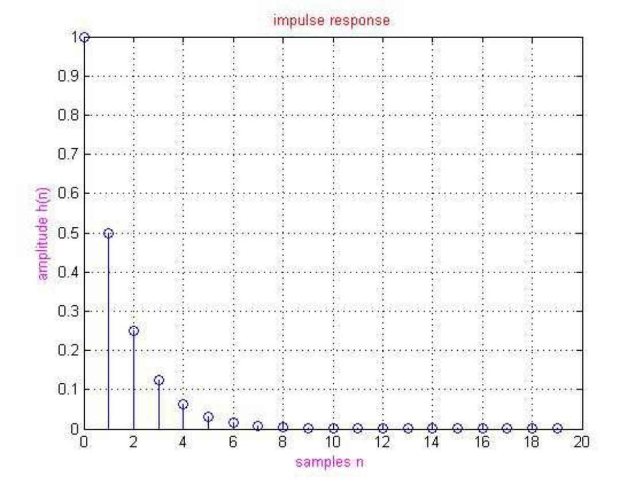
3. Impulse response of a given system

A discrete time LTI system (also called digital filters) as shown in Fig.2.1 is represented by

·         A linear constant coefficient difference equation, for example,

y[n] + a₁ y[n -1] - a₂ y[n - 2] = b₀ x[n] + b₁ x[n -1] + b₂ x[n - 2];

·         A system function H(z) (obtained by applying Z transform to the difference Equation

H (z) = Y(z) = b₀+b₁z^-1+b₂z^-2

                         X(z)    1+a₁z^-1+a₂z^-2

Given the difference equation or H(z), the impulse response of the LTI system is found using filter or impz MATLAB functions.

MATLAB Program:

b=input('numerator coefficients b = ');

a=input('denominator coefficients a = ');

n=input('enter length n = ');

[h,t] = impz(b,a,n);

disp(h);

stem(t,h);

xlabel('samples n ','color', 'm');

ylabel('amplitude h(n)','color','m');

title('impulse response','color','r');

grid on;

Result:

numerator coefficients b = [1]

denominator coefficients a = [1 -0.5]

enter length n = 20

1.0000    0.5000    0.2500    0.1250    0.0625    0.0313    0.0156    0.0078

0.0039    0.0020    0.0010    0.0005    0.0002    0.0001    0.0001    0.0000

0.0000    0.0000    0.0000    0.0000

4. Implementation of N point FFT:

Discrete Fourier Transform (DFT) is used for performing frequency analysis of discrete time signals. DFT gives a discrete frequency domain representation whereas the other transforms are continuous in frequency domain.

The N point DFT of discrete time signal x[n] is given by the equation

N-1	- j 2pkn
X (k ) = Σ x[n]e	N	;  k = 0,1,2,....N -1
n =0

Where N is chosen such that N ³ L , where L=length of x[n].

The inverse DFT allows us to recover the sequence x[n] from the frequency samples.

1		N -1	j 2pkn
x[n] =		Σ x[n]e	N	;  n = 0,1,2,....N -1
	N k =0

X(k) is a complex number (remember e^jw=cosω + jsinω). It has both magnitude and phase which are plotted versus k. These plots are magnitude and phase spectrum of x[n]. The ‘k’ gives us the frequency in formation.

Here k=N in the frequency domain corresponds to sampling frequency (fs). Increasing N, increases the frequency resolution, i.e., it improves the spectral characteristics of the sequence. For example if fs=8kHz and N=8 point DFT, then in the resulting spectrum, k=1 corresponds to 1kHz frequency. For the same fs and x[n], if N=80 point DFT is computed, then in the resulting spectrum, k=1 corresponds to 100Hz frequency. Hence, the resolution in frequency is increased.

Since N ³ L , increasing N to 8 from 80 for the same x[n] implies x[n] is still the same sequence (<8), the rest of x[n] is padded with zeros. This implies that there is no further information in time domain, but the resulting spectrum has higher frequency resolution. This spectrum is known as ‘high density spectrum’ (resulting from zero padding x[n]). Instead of zero padding, for higher N, if more number of points of x[n] are taken (more data in time domain), then the resulting spectrum is called a ‘high resolution spectrum’.

Algorithm:

1.      Input the sequence for which DFT is to be computed.

2.      Input the length of the DFT required (say 4, 8, >length of the sequence).

3.      Implement FFT algorithm.

4.      Plot the magnitude & phase spectra.

MATLAB Program:

%  This programme is for fast fourier transform in matlab.

%  Where y is the input argument and N is the legth of FFT . Let

%  y = [1 2 3 4 ];

y=input('enter input sequence:');

N= input('size of fft(e.g . 2,4,8,16,32):');

n=length(y);

p=log2(N);

Y=y;

Y=[Y, zeros(1, N - n)];

N2=N/2;

YY = -pi*sqrt(-1)/N2;

WW = exp(YY);

JJ = 0 : N2-1;

W=WW.^JJ;

for L = 1 : p-1

      u=Y(:,1:N2);

      v=Y(:,N2+1:N);

      t=u+v;

      S=W.*(u-v);

      Y=[t ; S];

      U=W(:,1:2:N2);

      W=[U ;U];

      N=N2;

      N2=N2/2;

end;

u=Y(:,1);

v=Y(:,2);

Y=[u+v;u-v];

Y

subplot(3,1,1)

stem(y);grid

title('input sequence y')

xlabel('n');

ylabel('Amplitude');

subplot(3,1,2)

stem(abs(Y));grid

title('Magnitude of FFT')

xlabel('N');

ylabel('Amplitude');

subplot (3,1,3)

stem(angle(Y));grid

title('phase of FFT')

xlabel('N');

ylabel('phase');

Result:

>> fft1

enter input sequence:[1 2 3 4 5 6 7]

size of fft(e.g . 2,4,8,16,32):8

Y =

28.0000

-9.6569 + 4.0000i

-4.0000 - 4.0000i

1.6569 - 4.0000i

4.0000

1.6569 + 4.0000i

-4.0000 + 4.0000i

-9.6569 - 4.0000i

Power Density Spectrum Using MATLAB

Algorithm:

1.  Generate a signal

2.  find DFT of the signal

3.    PSD is given by the formula

¥

y(n) =    Σ  x(k ) x(k - n)

k =-¥

where n = - (N-1)  to  (N-1)

PSD=  |Y(w)|²

Where Y(w) = fft of y(n)

Matlab program

%  computation of psd of signal corrupted with random noise

t = 0:0.001:0.6;

x = sin(2*pi*50*t)+sin(2*pi*120*t); 

y = x + 2*randn(size(t)); 

figure,plot(1000*t(1:50),y(1:50))

title('Signal Corrupted with Zero-Mean Random Noise')

xlabel('time (milliseconds)');

Y = fft(y,512);

%The power spectral density, a measurement of the energy at various frequencies, is: 

Pyy = Y.* conj(Y) / 512;

f = 1000*(0:256)/512; figure,plot(f,Pyy(1:257)) 

title('power spectrum of y');

xlabel('frequency (Hz)');

Implementation of FIR filter to meet given specifications

There are two types of systems – Digital filters (p erform signal filtering in time domain) and spectrum analyzers (provide signal representation in the frequency domain). The design of a digital filter is carried out in 3 steps- specifications, approximations and implementation.

DESIGNING AN FIR FILTER (using window method):

Method I:

Given the order N, cutoff frequency fc, sampling frequency fs and the window.

Step 1: Compute the digital cut-off frequency Wc (in the range -π < Wc < π, with π corresponding to fs/2) for fc and fs in Hz. For example let fc=400Hz, fs=8000Hz

Wc = 2*π* fc / fs  = 2* π * 400/8000 = 0.1* π radians

For MATLAB the Normalized cut-off frequency is in the range 0 and 1, where 1 corresponds to fs/2 (i.e.,fmax)). Hence to use the MATLAB commands wc = fc / (fs/2) = 400/(8000/2) = 0.1

Note: if the cut off frequency is in radians then the normalized frequency is computed as 

wc = Wc/ π

Step 2: Compute the Impulse Response h(n) of the required FIR filter using the given Window type and the response type (lowpass, bandpass, etc). For example given a rectangular window, order N=20, and a high pass response, the coefficients (i.e., h[n] samples) of the filter are computed using the MATLAB inbuilt command ‘fir1’ as

h =fir1(N, wc , 'high', boxcar(N+1));

Note: In theory we would have calculated h[n]=hd[n]×w[n], where hd[n] is the desired impulse response (low pass/ high pass,etc given by the sinc function) and w[n] is the window coefficients. We can also plot the window shape as stem(boxcar(N)).

Plot the frequency response of the designed filter h(n) using the freqz function and observe the type of response (lowpass / highpass /bandpass).

Method 2:

Given the pass band (wp in radians) and Stop band edge (ws in radians) frequencies, Pass band ripple Rp and stopband attenuation As.

Step 1: Select the window depending on the stopband attenuation required. Generally if As>40 dB, choose Hamming window. (Refer table )

Step 2: Compute the order N based on the edge frequencies as

Step 3: Compute the digital cut-off frequency Wc as 

Wc=(wp+ws)/2

Now compute the normalized frequency in the range 0 to 1 for MATLAB as

wc=Wc/pi;

Note: In step 2 if frequencies are in Hz, then obtain radian frequencies (for computation of tb and N) as 

wp=2*pi*fp/fs, ws=2*pi*fstop/fs, 

where fp, fstop and fs are the passband, stop band and sampling frequencies in Hz

Step 4: Compute the Impulse Response h(n) of the required FIR filter using N, selected window, type of response(low/high,etc) using ‘fir1’ as in step 2 of method 1.

MATLAB IMPLEMENTATION

FIR1 Function

B = FIR1(N,Wn) designs an N'th order lowpass FIR digital filter and returns the filter coefficients in length N+1 vector B. The cut-off frequency Wn must be between 0 < Wn<1.0, with 1.0 corresponding to half the sample rate. The filter B is real and has linear phase, i.e., even symmetric coefficients obeying B(k) = B(N+2-k), k = 1,2,...,N+1.

If Wn is a two-element vector, Wn = [W1 W2], FIR1 returns an order N bandpass filter with passband W1 < W < W2. B = FIR1(N,Wn,'high') designs a highpass filter. B = FIR1(N,Wn,'stop') is a bandstop filter if Wn = [W1W2]. If Wn is a multi-element vector, Wn = [W1 W2 W3 W4 W5 ... WN], FIR1 returns an order N multiband filter with bands 0 < W < W1, W1 < W < W2, ..., WN < W < 1. FREQZ Digital filter frequency response. [H,W] = FREQZ(B,A,N) returns the N-point complex frequency response vector H and the N-point frequency vector W in radians/sample of the filter whose numerator and denominator coefficients are in vectors B and A. The frequency response is evaluated at N points equally spaced around the upper half of the unit circle. If N isn't specified, it defaults to 512.

For FIR filter enter A=1 and B = h[n] coefficients. Appropriately choose N as 128, 256, etc

Window

Transition

Width Δ ω

Min. Stop band

Matlab

Name

Approximate

Exact values

Attenuation

Command

Rectangular

4 π

1.8 π

21db

B = FIR1(N,Wn,boxcar)

M

M

Bartlett

8π

6.1 π

25db

B = FIR1(N,Wn,bartlett)

M

M

Hanning

8π

6.2 π

44db

B = FIR1(N,Wn,hanning)

M

M

Hamming

8π

6.6π

53db

B= FIR1(N,Wn,hamming)

M

M

Blackman

12 π

11 π

74db

B = FIR1(N,Wn,blackman)

M

M

Matlab Program:

%Method 2: the following program gives only the design of the FIR filter for implementation continue with the next program (after h[n]) %input data to be given: Passband & Stopband frequency

%  Data given: Passband ripple & stopband attenuation As. If As>40 dB, Choose hamming

clear

wpa=input('Enter passband edge frequency in Hz'); wsa= input('Enter stopband edge frequency in Hz'); ws1= input('Enter sampling frequency in Hz');

%Calculate transmission BW,Transition band tb,order of the filter

wpd=2*pi*wpa/ws1;

wsd=2*pi*wsa/ws1;

tb=wsd-wpd;

N=ceil(6.6*pi/tb)

wc=(wsd+wpd)/2;

%compute the normalized cut off frequency

wc=wc/pi;

%calculate & plot the window

hw=hamming(N+1);

stem(hw);

title('Fir filter window sequence- hamming window');

%find h(n) using FIR

h=fir1(N,wc,hamming(N+1));

%plot the frequency response

figure(2);

[m,w]=freqz(h,1,128);

mag=20*log10(abs(m));

plot(ws1*w/(2*pi),mag);

title('Fir filter frequency response');

grid;

%generate simulated input of 50, 300 & 200 Hz, each of 30 points

n=1:30;

f1=50;f2=300;f3=200;fs=1000;

x=[];

x1=sin(2*pi*n*f1/fs);

x2=sin(2*pi*n*f2/fs);

x3=sin(2*pi*n*f3/fs);

x=[x1 x2 x3];

subplot(2,1,1);

stem(x);

title('input');

%generate o/p

%y=conv(h,x);

y=filter(h,1,x);

subplot(2,1,2);

stem(y);

title('output');

Result:

Enter passband edge frequency in Hz100

Enter stopband edge frequency in Hz200

Enter sampling frequency in Hz1000

N = 33

Plots are as in Fig.11.1 and 11.2

Inference:

Notice the maximum stopband attenuation of 53 dB from plot 11.2

%Design and implementation of FIR filter Method 1

%generate filter coefficients for the given %order & cutoff Say N=33, fc=150Hz, %fs=1000 Hz, Hamming window

h=fir1(33, 150/(1000/2),hamming(34));

%generate simulated input of 50, 300 & 200 Hz, each of 30 points

n=1:30;

f1=50;f2=300;f3=200;fs=1000;

x=[];

x1=sin(2*pi*n*f1/fs);

x2=sin(2*pi*n*f2/fs);

x3=sin(2*pi*n*f3/fs);

x=[x1 x2 x3];

subplot(2,1,1);

stem(x);

title('input');

%generate o/p

%y=conv(h,x);

y=filter(h,1,x);

subplot(2,1,2);

stem(y);

title('output');

Result:

Plots are in Fig.11.3 & 11.4

Notice that freqs below 150 Hz are passed & above 150 are cutoff

FIR filter design using Kaiser window:

disp('FIR filter design  using Kaiser window');

M = input ('enter the length of the filter = ');

beta= input ('enter the value of  beta = ');

Wc = input ('enter the digital cutoff frequency');

Wn= kaiser(M,beta);

disp('FIR Kaiser window coefficients');

disp(Wn);

hn = fir1(M-1,Wc,Wn);

disp('the unit sample response of FIR filter is hn=');

disp(hn);

freqz(hn,1,512);

grid on;

xlabel('normalized frequency');

ylabel('gain in db');

title('freq response of FIR filter');

Result:

FIR filter design  using Kaiser window

enter the length of the filter = 30

enter the value of  beta = 1.2

enter the digital cutoff frequency.3

FIR Kaiser window coefficients

0.7175     0.7523      0.7854    0.8166    0.8457    0.8727    0.8973    0.9195

0.9392     0.9563      0.9706    0.9822    0.9909    0.9967    0.9996    0.9996

0.9967     0.9909      0.9822    0.9706    0.9563    0.9392    0.9195    0.8973

0.8727	0.8457	0.8166	0.7854		0.7523	0.7175
the unit sample response of FIR filter is hn=
Columns 1 through 5
0.0141	0.0028	-0.0142	-0.0224	-0.0117
Columns 6 through 10
0.0133	0.0333	0.0277	-0.0072	-0.0495
Columns 11 through 15
-0.0614  -0.0140   0.0895   0.2097   0.2900
Columns 16 through 20
0.2900	0.2097	0.0895	-0.0140	-0.0614
Columns 21 through 25
-0.0495  -0.0072   0.0277   0.0333   0.0133
Columns 26 through 30
-0.0117	-0.0224	-0.0142	0.0028		0.0141

Implementation of IIR filter

There are two methods of stating the specifications as illustrated in previous program. In the first program, the given specifications are directly converted to digital form and the designed filter is also implemented. In the last two programs the butterworth and chebyshev filters are designed using bilinear transformation (for theory verification).

Method I: Given the order N, cutoff frequency fc, sampling frequency fs and the IIR filter type (butterworth, cheby1, cheby2).

Step 1: Compute the digital cut-off frequency Wc (in the range -π < Wc < π, with

π    corresponding to fs/2) for fc and fs in Hz. For example let fc=400Hz, fs=8000Hz Wc = 2*π* fc / fs = 2* π * 400/8000 = 0.1* π radians

For MATLAB the Normalized cut-off frequency is in the range 0 and 1, where 1 corresponds to fs/2 (i.e.,fmax)). Hence to use the MATLAB commands wc =  fc / (fs/2) = 400/(8000/2) = 0.1

Note: if the cut off frequency is in radians then the normalized frequency is computed as wc = Wc / π

Step 2: Compute the Impulse Response [b,a] coefficients of the required IIR filter and the response type (lowpass, bandpass, etc) using the appropriate butter, cheby1, cheby2 command. For example given a butterworth filter, order N=2, and a high pass response, the coefficients [b,a] of the filter are computed using the MATLAB inbuilt command ‘butter’ as [b,a] =butter(N, wc , 'high'); Given the pass band (Wp in radians) and Stop band edge (Ws in radians) frequencies, Pass band ripple Rp and stopband attenuation As.

Step 1: Since the frequencies are in radians divide by π to obtain normalized frequencies to get wp=Wp/pi and ws=Ws/pi. If the frequencies are in Hz (note: in this case the sampling frequency should be given), then obtain normalized frequencies as wp=fp/(fs/2), ws=fstop/(fs/2), where fp, fstop and fs are the passband, stop band and sampling frequencies in Hz

Step 2: Compute the order and cut off frequency as[N, wc] = BUTTORD(wp, ws, Rp, Rs)

Step 3: Compute the Impulse Response [b,a] coefficients of the required IIR filter and the response type as [b,a] =butter(N, wc , 'high');

IMPLEMENTATION OF THE IIR FILTER

1.      Once the coefficients of the IIR filter [b,a] are obtained, the next step is to simulate an input sequence x[n], say input of 100, 200 & 400 Hz (with sampling frequency of fs), each of 20/30 points. Choose the frequencies such that they are >, < and = to fc.

2.      Filter the input sequence x[n] with Impulse Response, to obtain the output of the filter y[n] using the ‘filter’ command.

3.      Infer the working of the filter (low pass/ high pass, etc).

MATLAB IMPLEMENTATION

BUTTORD Butterworth filter order selection.

[N, Wn] = BUTTORD(Wp, Ws, Rp, Rs) returns the order N of the lowest order digital Butterworth filter that loses no more than Rp dB in the passband and has at least Rs dB of attenuation in the stopband. Wp and Ws are the passband and stopband edge frequencies, normalized from 0 to 1 (where 1 corresponds to pi radians/sample). For example,

Bandpass:   Wp = [.2 .7], Ws = [.1 .8]   Bandstop:   Wp = [.1 .8], Ws = [.2 .7]

BUTTORD also returns Wn, the Butterworth natural frequency (or, the "3 Db frequency") to use with BUTTER to achieve the specifications.

[N, Wn] = BUTTORD(Wp, Ws, Rp, Rs, 's') does the computation for an analog filter, in which case Wp and Ws are in radians/second.When Rp is chosen as 3 dB, the Wn in BUTTER is equal to Wp in BUTTORD.

BUTTER Butterworth digital and analog filter design.

[B,A] = BUTTER(N,Wn) designs an Nth order lowpass digital Butterworth filter and returns the filter coefficients in length N+1 vectors B (numerator) and A (denominator). The coefficients are listed in descending powers of z.

The cutoff frequency Wn must be 0.0 < Wn < 1.0, with 1.0 corresponding to half the sample rate. If Wn is a two-element vector, Wn = [W1 W2], BUTTER returns an order 2N bandpass filter with passband W1<W < W2.

[B,A] = BUTTER(N,Wn,'high') designs ahighpass filter. [B,A] = BUTTER(N,Wn,'stop') is a bandstop filter if Wn = [W1 W2].

BUTTER(N,Wn,'s'), BUTTER(N,Wn,'high','s') and BUTTER(N,Wn,'stop','s') design analog Butterworth filters. In this case, Wn is in [rad/s] and it can be greater than 1.0.

Matlab Program (Design & implementation)

%generate filter coefficients for the given %order & cutoff %Say N=2, fc=150Hz, %fs=1000 Hz, butterworth filter

[b,a]=butter(2, 150/(1000/2));

%generate simulated input of 100, 300 & 170 Hz, each of 30 points

n=1:30;

f1=100;f2=300;f3=170;fs=1000;

x=[];

x1=sin(2*pi*n*f1/fs);

x2=sin(2*pi*n*f2/fs);

x3=sin(2*pi*n*f3/fs);

x=[x1 x2 x3];

subplot(2,1,1);

stem(x);

title('input');

%generate o/p

y=filter(b,a,x);

subplot(2,1,2);

stem(y);

title('output');

Result:

Plot is in Fig. 1, which shows that 100 Hz is passed, while 300 is cutoff and 170 has slight attenuation.

Note: If fp,fstp,fs, rp,As are given then use [N,wc]=buttord(2*fp/fs,2*fstp/fs,rp,As) [b,a]=butter(N,wc);

If wp & ws are in radians [N,wc]=buttord(wp/pi,ws/pi,rp,As) [b,a]=butter(N,wc);

If wc is in radians & N is given

[b,a]=butter(N,wc/pi);                                                       

For a bandpass output

wc=[150/(1000/2) 250/(1000/2)];

[b,a]=butter(4, wc);

Plot is in fig.2 where only 170 is passed, while 100 & 300 are cutoff.

Fig1. Low Pass IIR filter (butterworth) output

Fig 2. IIR Output for Band Pass (150-250 Hz)

Programs for designing of IIR filters (for theory practice): BUTTERWORTH

%    Butterworth filter: Given data: rp=1, rs=40, w1=800, w2=1200,ws=3600;

rp=1, rs=40, w1=800, w2=1200,ws=3600;

%  Analog frequency

aw1=2*pi*w1/ws;

aw2=2*pi*w2/ws;

% Prewrapped frequency

pw1 = 2*tan(aw1/2); pw2 = 2*tan(aw2/2);

%Calculate order and cutoff freq

[n,wc]= buttord (pw1,pw2,rp,rs,'s');        

%  analog filter transfer

[b,a] = butter(n,wc,'s');

% obtaining the digital filter using bilinear transformation fs=1;

[num,den]= bilinear(b,a,fs);

% plot the frequency response

[mag,freq1]=freqz(num,den,128);

freq=freq1*ws/(2*pi);

m = 20*log10(abs(mag));

plot(freq,m);

grid;

Result:

rp = 1     rs = 40     w1 = 800     w2 = 1200

CHEBYSHEV FILTER:

%Given data

rp=1,rs=40,w1=800,w2=1200,ws=3600

%Analog frequencies

aw1= 2*pi*w1/ws;

aw2=2*pi*w2/ws;

%  Prewrapped frequency assuming T=1/fs pw1 = 2*tan(aw1/2);

pw2 = 2*tan(aw2/2);

[n,wc]= cheb1ord (pw1,pw2,rp,rs,'s');

[b,a] = cheby1(n,rp,wc,'s');

%obtaining the digital filter using bilinear transformation fs=1;

[num,den]= bilinear(b,a,fs);

%plot the frequency response

[mag,freq1]=freqz(num,den,128);

freq=freq1*ws/(2*pi);

m = 20*log10(abs(mag));

plot(freq,m);

grid;

Result:  

rp = 1   rs = 40    w1 = 800 w2 = 1200      ws = 360

Generation of sinusoidal wave using recursive difference equation

There exists different techniques to generate a sine wave on a DSP processor. Using a lookup table, interpolation, polynomials, or pulse width modulation are some of these techniques utilized to generate a sine wave. When a slightly sufficient processing power is considered, it is possible to utilize another technique which makes use of an IIR filter.

In this technique, a second order IIR filter as shown in Figure 1 is designed to be marginally stable which is an undesirable situation for a normal filtering operation. For this second order filter to be marginally stable, its poles are located in the unit circle. After choosing the suitable filter coefficients for the filter to be marginally stable, a unit impulse is applied to the filter as an input at time t = 0, and then the input is disconnected. Then the filter starts to oscillate with a fixed frequency.

The difference equation of the second order filter shown in Figure 1 will be:

Where F0 is the frequency, Fs is the sampling frequency and A is the amplitude of the sine wave

Matlab Program

%  Generation of sine wave using recursive difference equation or IIRfilter 

%fs = sampling rate

%  t = time in sec

%f0 = frequency

%  A =amplitude 

A = 2;

t=0.1;

fs = 5000; 

f0=50; 

length = fs*t;

y = zeros(1,length); 

impulse = zeros(1,length); 

impulse(1) = 1;

%  frequency coefficients

%  difference equation of form y[n]= -a1 y[n-1] -a2 y[n-2] + b0 impulse[n]

%  a1 = -2cos(2*pi*f0/fs), a2= 1, b0 = Asin(2*pi*f0/fs)

a1 = -2*cos(2*pi*f0/fs)

a2 = 1;

b0 = A*sin(2*pi*f0/fs)

y(1)= 0;

y(2)= b0;

for i=3:length

y(i)=  b0* impulse(i)- a1*y(i-1) - a2* y(i-2);

end

plot (y);

title('Sinusoidal waveform')

xlabel('samples n');

ylabel('y(n)');

Generation of  DTMF signals

Dual-tone Multi-Frequency (DTMF) signaling is the basis for voice communications control and is widely used worldwide in modern telephony to dial numbers and configure switchboards. It is also used in systems such as in voice mail, electronic mail and telephone banking.

A DTMF signal consists of the sum of two sinusoids - or tones - with frequencies taken from two mutually exclusive groups. These frequencies were chosen to prevent any harmonics from being incorrectly detected by the receiver as some other DTMF frequency. Each pair of tones contains one frequency of the low group (697 Hz, 770 Hz, 852 Hz, 941 Hz) and one frequency of the high group (1209 Hz, 1336 Hz, 1477Hz) and represents a unique symbol. The frequencies allocated to the push-buttons of the telephone pad are shown below:

	1209Hz	1336Hz	1477 Hz
697Hz		ABC	DEF
	1	2	3
770 Hz	GHI	JKL	MNO
	4	5	6
852Hz	PQRS	TUV	WXYZ
	7	8	9
941 Hz	*	0	#

We will right the program to generate and visualize the DTMF tones for all 12 Symbols. 

Also we will estimate its energy content using Gortzet’s Algorithm

The minimum duration of a DTMF signal defined by the ITU standard is 40 ms. Therefore, there are at most 0.04 x 8000 = 320 samples available for estimation and detection. The DTMF decoder needs to estimate the frequencies contained in these short signals.

One common approach to this estimation problem is to compute the Discrete-Time Fourier Transform (DFT) samples close to the seven fundamental tones. For a DFT-based solution, it has been shown that using 205 samples in the frequency domain minimizes the error between the original frequencies and the points at which the DFT is estimated.

At this point we could use the Fast Fourier Transform (FFT) algorithm to calculate the DFT. However, the popularity of the Goertzel algorithm in this context lies in the small number of points at which the DFT is estimated. In this case, the Goertzel algorithm is more efficient than the FFT algorithm.

Plot Goertzel's DFT magnitude estimate of each tone on a grid corresponding to the telephone pad.

MATLAB Program

% generating all 12 frequencies

symbol = {'1','2','3','4','5','6','7','8','9','*','0','#'};

lfg = [697 770 852 941]; % Low frequency group 

hfg = [1209 1336 1477]; % High frequency group

f    = []; 

for c=1:4,

for r=1:3,

f = [ f [lfg(c);hfg(r)] ]; end

end 

f'

% Generate the DTMF tones

Fs  = 8000;% Sampling frequency 8 kHz

N = 800;% Tones of 100 ms

t = (0:N-1)/Fs; % 800 samples at Fs 

pit = 2*pi*t;

tones = zeros(N,size(f,2));

for toneChoice=1:12,

% Generate tone

tones(:,toneChoice) = sum(sin(f(:,toneChoice)*pit))';

%  Plot tone s

ubplot(4,3,toneChoice),plot(t*1e3,tones(:,toneChoice));

title(['Symbol "', symbol{toneChoice},'":

[',num2str(f(1,toneChoice)),',',num2str(f(2,toneChoice)),']'])

set(gca, 'Xlim', [0 25]);

ylabel('Amplitude');

if toneChoice>9, xlabel('Time (ms)'); end

end

set(gcf, 'Color', [1 1 1], 'Position', [1 1 1280 1024])

 annotation(gcf,'textbox', 'Position',[0.38 0.96 0.45 0.026],...

'EdgeColor',[1 1 1],...

'String', '\bf Time response of each tone of the telephone pad', ...

'FitHeightToText','on');

%  estimation of DTMF tone using Gortzel's Algorithm 

Nt = 205;

original_f = [lfg(:);hfg(:)] % Original frequencies

k = round(original_f/Fs*Nt); % Indices of the DFT

estim_f = round(k*Fs/Nt)      % Frequencies at which the DFT is estimated

tones = tones(1:205,:);

figure,

for toneChoice=1:12,

%  Select tone tone=tones(:,toneChoice);

%  Estimate DFT using Goertzel

ydft(:,toneChoice) = goertzel(tone,k+1); % Goertzel use 1-based indexing

%  Plot magnitude of the DFT 

subplot(4,3,toneChoice),stem(estim_f,abs(ydft(:,toneChoice))); title(['Symbol "', symbol{toneChoice},'":

[',num2str(f(1,toneChoice)),',',num2str(f(2,toneChoice)),']'])

set(gca, 'XTick', estim_f, 'XTickLabel', estim_f, 'Xlim', [650 1550]); ylabel('DFT Magnitude');

if toneChoice>9, xlabel('Frequency (Hz)'); end 

end

set(gcf, 'Color', [1 1 1], 'Position', [1 1 1280 1024]) a

nnotation(gcf,'textbox', 'Position',[0.28 0.96 0.45 0.026],...

'EdgeColor',[1 1 1],...

'String', '\bf Estimation of the frequencies contained in each tone of the telephone pad using Goertzel', ... 'FitHeightToText','on');

Interpolation, decimation and I/D sampling rate converters

Multirate : Changing the Sampling Rate of the Discrete Time Signal.

The process of converting a signal from a given rate to a different rate is called sampling rate conversion.

Systems that employ multiple sampling rates in the processing of digital signals are called multirate digital signal processing systems.

Can be accomplished in two ways:

Adv: New sampling rate can be arbitrarily selected

Disadv: Signal distortion is introduced by

·          D/A converter in signal reconstruction

·          Quantization effects in A/D converter

Changing the sampling rate in digital domain --Multirate

Fundamental operations in multirate signal processing are

1)  Downsampling (Decimation)

2)  Upsampling(Interpolation )

Decimation is the process of decreasing the sampling rate by a factor of M i.e. from Fs to Fs / M

Down sampling : by a factor of M is achieved by discarding M-1 samples for every M samples.

This combined operation of filtering and down sampling is called as decimation.

The rate compressor reduces the sampling rate from F_s to F_s / M

To prevent aliasing at lower rate, digital filter is used to band limit the i/p signal to less than F_s/2M. (new folding frequency).

Sampling rate reduction is achieved by discarding M-1 samples for every M samples of filtered signal W(n).

INTERPOLATION

Process of increasing the sampling rate of the signal by a factor of L i.e. from F _s to LF_s Upsampling by a factor L means inserting L-1 zeros between two samples.

In matlab we can use function resample() to achieve interpolation as well as decimation.

MATLAB program:

%  % m-file to illustrate simple interpolation and

%  decimation operations

%  File name:

%

Fs=input('Enter Sampling Frequency:'); % sampling frequency

I= input('interpolation factor:');

A=1.5; % relative amplitudes

B=1;

f1=50; % signal frequencies

f2=100;

t=0:1/Fs:1; % time vector

x=A*cos(2*pi*f1*t)+B*cos(2*pi*f2*t); % generate signal

y=resample(x,I,1); % interpolate signal by 4

stem(x(1:100)) % plot original signal

xlabel('Discrete time, nT ')

ylabel('Input signal level')

figure

stem(y(1:400)) % plot interpolated signal.

xlabel('Discrete time 4 X nT')

ylabel('Interpolated output signal level')

D=input('Enter the decimation factor:');

y1=resample(x,1,D);

figure

stem(y1(1:50)) % plot decimated signal.

xlabel('Discrete time nT/2')

ylabel('Decimated output signal level')

Result

>> decimation

Enter Sampling Frequency:1000

interpolation factor:4

Enter the decimation factor:2